
Strategy 3: Set targets and design monitoring

“Although it is difficult to predict the exact amount of stress that will trigger a tipping point, warning signs that precede the tipping point can be instrumental in avoiding collapse.” – Selkoe et al. 2015
Background
Whether you seek to avoid an undesirable regime shift or you are trying to restore a system that has already shifted, knowing how close your ecosystem is to a tipping point is crucial. This includes knowing what trajectory your managed system is on, where it is currently and where you want it to be relative to the tipping point.
Here we review how indicators can help you recognize when your ecosystem may be approaching a tipping point, how this emerging science can inform the design of monitoring programs, and how ecological and social information about tipping points can assist you in setting management targets. Below are three definitions that will help you as you navigate through this strategy.
A target is a specific, measurable outcome you are trying to reach.
A benchmark is an intermediate, measurable outcome that can signal progress toward your target.
A limit is a specific, measurable outcome to be avoided.
Strategy 3a. Identify early warning indicators that signal approach of a tipping point
What does this mean?
When assembled effectively, a suite of social and ecological indicators can help managers detect changes in ecosystem status and trends, providing them with the information necessary to evaluate their current and past policy decisions as well as plan for the future.
Indicators help managers establish monitoring benchmarks that can be used to judge when a management target has been reached (Samhouri et al. 2011, 2012). These targets can be set by identifying particular ecosystem thresholds through quantitative analysis or through peoples' stated or revealed preferences for particular ecosystem conditions (Samhouri et al. 2013). Active monitoring of indicators in relation to these targets can inform adaptive management.
Early warning indicators are a specific type of indicator that provides information in advance of an ecosystem shift. These indicators are most effective if they provide information that allows managers to be able to anticipate shifts with sufficient time to respond.

Planting rose bushes in grape vineyards is an example of establishing an early warning indicator system. Roses and grapevines are both susceptible to the same fungus, but roses are more sensitive, so will respond first to the presence of the fungus. Once the roses start to show signs of the fungus they function as an early warning indicator to grape farmers that they need to act quickly to prevent the spread of the fungus to their grapevines.
Why is it important?
The “timely information” that early warning indicators provide could ultimately dictate whether or not a manager has enough lead time to effectively take action to avoid a looming ecosystem shift (Biggs et al. 2009). Incorporating early warning indicators into your ecosystem monitoring portfolio can therefore help you to avoid undesirable shifts, plan for unavoidable changes, and track progress toward management targets. This kind of information collection and feedback is essential to any adaptive management framework, and especially so when there is a risk of dramatic ecosystem level change or when mitigation is not an option.
How do you do it?
Complex systems theory predicts that, under certain conditions, generic "early warning" signs should presage critical transitions from one state of a system to another (Dakos et al. 2008, Scheffer et al. 2009). Early warning indicators, which constitute different statistical properties of time series or spatial data (Table 5, from Foley et al. 2015 with permission), have potential application in a wide variety of situations where the change in state is characterized by hysteresis. Litzow and Hunsicker (2016) highlight the importance of testing for nonlinear dynamics or hysteresis before attempting to apply early warning indicators in monitoring a system. From analysis of northeast Pacific Ocean time series and literature review across many different study systems, they found that systems with evidence for nonlinear dynamics or hysteresis generally supported theoretical early warning indicator predictions, while those with linear or unknown dynamics did not. While their potential is alluring, some scientists caution against use of these indicators without thorough understanding of the underlying system dynamics (e.g., Boettiger and Hastings 2012). Boettiger and Hastings suggest it is unlikely that general indicators exist across systems because the context in which a system approaches a threshold is likely to be unique. Instead, they push for data-driven exploration and experimentation within systems to identify system-specific characteristics of impending thresholds.
Major categories of early warning indicators (EWI)
Critical slowing down and flickering. As a system approaches a threshold, the time it takes to recover from a disturbance increases due to loss of resilience (Scheffer et al. 2009) and the structure and/or function of the ecosystem starts to alternate between two states over a short time period (Dakos et al. 2012).
Autocorrelation. Change across ecosystems tends to become correlated in space and time prior to a tipping point (Biggs et al, 2009; Kéfi et al. 2014). This shift occurs when large-scale dynamics, such as climate shifts, dominate ecosystem response rather than within system feedbacks that maintained stability and functioning prior to ecosystem decline.
Variance. The response of ecosystem components to drivers becomes more variable as a threshold is approached. Increased variance can be detected with little underlying knowledge of “normal” ecosystem dynamics (Carpenter and Brock, 2006; Litzow et al. 2013), and can be detected in spatial and temporal analyses (Donangelo et al. 2010).
To learn more about these Early Warning Indicators, visit the Early Warning Signals Toolbox website: http://www.early-warning-signals.org/
“Critical slowing down,” in which the time it takes a system to recover from a disturbance increases due to loss of resilience, is thought to be one of the most robust early warning indicators of an impending ecological threshold (Scheffer et al. 2009). However, while early warning indicators hold promise, researchers are just beginning to test them in experimental and natural biological systems (reviewed in Litzow & Hunsicker 2016). For example, rising spatial variance in fisheries catch time-series was found to be a precursor to historical fishing collapses in the Gulf of Alaska and the Bering Sea (Litzow et al. 2013). Similarly, variance in macroalgal cover, fish diversity, and other coral reef ecosystem status metrics appear to precede tipping points on coral reefs (McClanahan et al. 2011, Karr et al. 2015)
How useful early warning indicators are partly depends on the dataset to which they are applied. In general, you are seeking an indicator that has a good signal to noise ratio and which is sensitive to the purported driver(s) of ecosystem change. Species with short generation times such as zooplankton, for example, might provide earlier warning of a climate-driven ecosystem transition than larger, slower-growing species, however, their population dynamics may also be so noisy that trends in statistical properties like variance are difficult to detect.
Beyond generic statistical indicators, knowledge of the dynamics of your ecosystem can also reveal appropriate early warning indicators. For example, we know that diversity and functional redundancy at multiple levels (e.g., within species, across species, and across trophic groups) can affect a system’s resilience to change. As components of the ecosystem are compromised or lost, the system may lose resilience and become more prone to crossing a tipping point with the next shock or stressor (Briske et al. 2006, Brandl and Bellwood 2014). In well studied systems, it is possible to relate specific changes in diversity and ecological functions to system resilience and to identify proxies or indicators of those changes for monitoring.
For example, scientists and managers are currently developing ecosystem indicators for Caribbean coral reefs based on threshold responses of the ecosystem to overfishing (Karr et al. 2015). Applying a method piloted in the Indian Ocean (McClanahan et al. 2011), the team analyzed monitoring data from 2,001 Caribbean coral reef sites that span a gradient of fishing intensity and reef condition. Karr and colleagues found that lower fish biomass was correlated with several other commonly monitored metrics of ecosystem condition, including decreased fish diversity and coral cover, and increased macroalgal cover. In this system, reductions in fish biomass appear to be good indicators of forthcoming ecosystem shifts (Figure 16, adapted from Karr et al. 2015 with permission). Coral cover, on the other hand, which has historically been used as an indicator of reef health, is associated with quite low levels of fish biomass, suggesting it’s a lagging rather than leading indicator of coral reef tipping points.
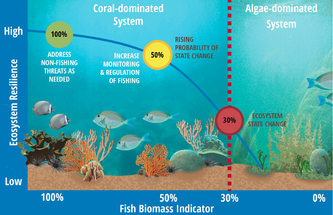
Figure 18, based on Karr et al. 2015. Coral reef studies suggest that a number of coral reef system traits related to resilience (e.g., the proportion of herbivorous fishes, the number of fish species, and urchin density) show steep declines when fish biomass falls below 50% of unfished biomass. Unfished density can be estimated from established local no-take reserves. A tiered approach to risk might set response plans based on these targets (colored circles)
Summary of methods for developing and analyzing early warning indicators of nonlinear ecosystem change
Multivariate autoregressive state-space model (MARSS) |
|
| Output | Identifies how non-linear changes are related to biotic processes and changes in outside drivers |
| Quantifies interaction strength between driver(s) and response variable(s) | |
| Strengths | Accommodates multivariate datasets |
| Identifies drivers and ecosystem responses that could serve as early warning indicators | |
| Quantifies interaction strengths among drivers | |
| Weaknesses | Correlational |
| Requires significant data input | |
| More information & examples | Zuur et al. (2003), Hampton and Schindler (2006), Holmes et al. (2012), Hampton et al. (2013) |
| Software & code examples | MAR1 and MARSS R packages; Matlab code (Ives et al. 2003) |
Structural equation modeling (SEM) |
|
| Output | Predicts how an ecosystem is likely to respond to changes in direct and indirect drivers |
| Strengths | Predicts directionality and strength of relationship between driver and ecosystem response |
| Accommodates wide range of data types | |
| Allows for incorporation of feedback loops and two-way interactions | |
| Weaknesses | Requires significant data inputs |
| Requires a priori understanding of ecosystem | |
| Does not incorporate non-linearities in relationships | |
| More information & examples | Grace (2008), Grace et al. (2010), Thrush et al. (2012), Fox et al. (2015) |
| Software & code examples | sem R package |
Regime shift indicators (e.g., variance; autocorrelation; flickering) |
|
| Output | Provides early warning of threshold dynamics and regime shifts in spatial and temporal data sets |
| Strengths | Accommodates wide range of data, including spatial and temporal data |
| Allows early identification of threshold dynamics and regime shifts | |
| Weaknesses | Requires significant data inputs |
| Most examples retrospective | |
| May not be transferable across systems | |
| More information & examples | Dakos et al (2010, 2012), (Veraart et al. 2012), Litzow et al (2013), |
| Software & code examples | nlme R package |
For additional resources, code, and methods that can be used to identify early warning indicators, visit The Early Warning Signals Toolbox website: http://www.early-warning-signals.org/
Strategy 3b. Use social preferences, risk tolerance and social and ecological thresholds to inform target-setting
What does this mean?
Target-setting requires integrating people’s values and tolerance for risk with the best available science to make a judgment about where you want the system to be. Defining thresholds and setting precautionary buffers can be viewed as setting the boundaries of a system’s “safe operating space”, in which the risk of crossing an unwanted tipping point is considered acceptable and resilience is high.
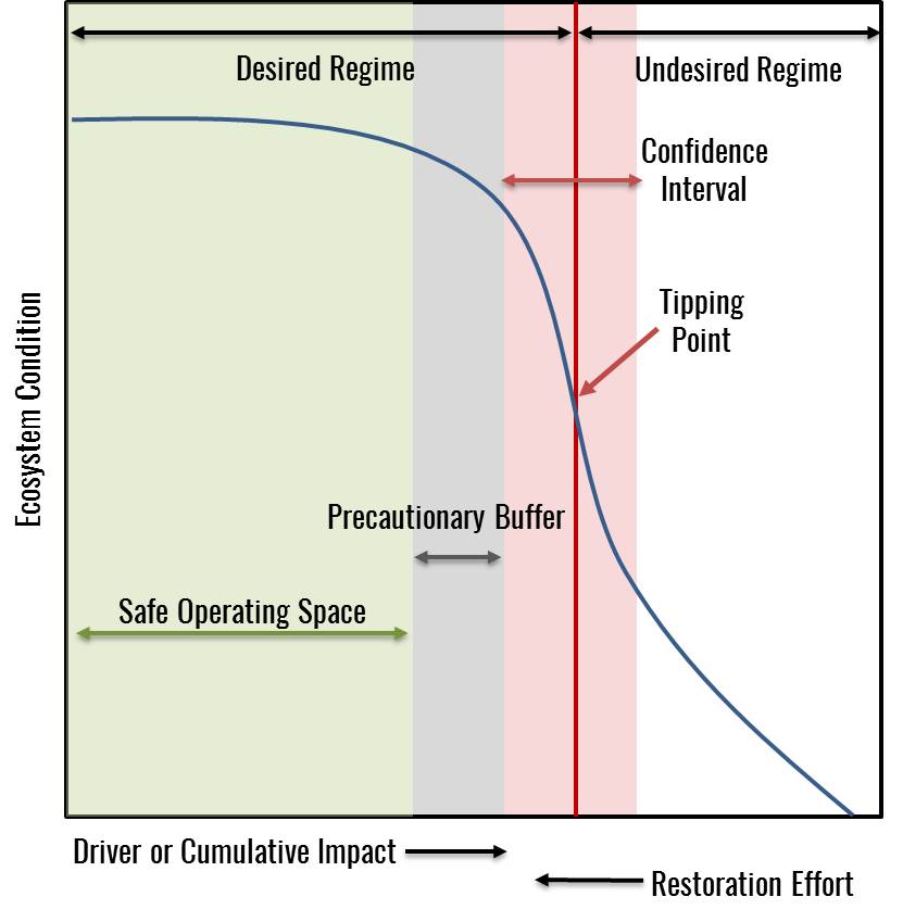
Figure 19, adapted from Selkoe et al. 2015 with permission. The safe operating space (green) for management represents the range of driver levels with a tolerable level of risk of tipping into an undesired regime or ecosystem state and adequate to high resilience. If the risks associated with crossing the tipping point or costs of mitigation are very high or if the location of the tipping point is highly uncertain, the precautionary buffer (blue) should be increased.
Scientifically quantified thresholds can provide important reference points in that process, as, for example, maximum sustainable yield determinations do in fisheries quota setting. Maximum sustainable yield (MSY) is determined through stock assessment methods that consider the nonlinear relationships between a species’ biomass, carrying capacity, and growth rate. It represents a limit for the amount of fishing a population could sustain under prevailing ecological and environmental conditions, fishery technological characteristics (e.g., gear selectivity), and the distribution of catch among fleets—“as reduced by any relevant economic, social, or ecological factor.”. The final target, optimum yield (OY), refers to the amount of fish that provides the greatest overall benefit to the Nation, accounting for food production, recreational opportunities, and protection of marine ecosystems but never exceeding sustainable levels, defined by MSY. The definitions of both maximum sustainable yield and optimum yield contemplate consideration of both species-specific and ecosystem thresholds and societal perceptions of risk. Current management guidance (NOAA’s National Standards Guidelines) calls for MSY and OY to provide the basis for both status determination criteria—criteria that define when a stock is overfished or subject to overfishing—and required catch limits for each fishery. In other words they are directly linked to the legally harvestable portion of fishery resources and the regulatory thresholds beyond which rebuilding plans are required and accountability measures (i.e., consequences) are triggered. In this way, the regulatory system calls for incorporation of social, economic, and ecosystem considerations.
Why is it important?
Setting targets helps you, as a manager:
- Track your progress;
- Anticipate upcoming shifts;
- Trigger appropriate, proactive management actions; and
- Evaluate the success of those actions.
It also allows the public and policymakers to do the same, leading to greater public understanding and enhanced accountability. In a system that is prone to tipping points and potentially high uncertainty, targets can help you track whether your management is maintaining the system within the determined safe operating space or moving it along a desirable trajectory.
How do you do it?
Once you have identified the known thresholds (Strategy 1), people’s social preferences and risk tolerance (Strategy 2), and indicators of these changes (Strategy 3a), the next phase is to identify your targets in relation to the indicators you are monitoring. Below we describe a few examples that illustrate the approaches people have used.
2020 targets for the Puget Sound
In 2011, the Puget Sound Partnership (“Partnership”) employed a science-based decision making process for understanding environmental, social, and economic trade-offs associated with the human activity and management decisions that affect the health of Puget Sound. Using the Integrated Ecosystem Assessment (IEA) framework, the Partnership identified and adopted ecosystem recovery targets that would help them work toward certain desired conditions for the ecosystem by 2020. First, the Partnership identified a number of indicators of the system. Scientific advisors then developed potential targets for those indicators based on thresholds, and/or baseline reference conditions. Stakeholders then provided perspectives about socially acceptable definitions of recovery by 2020, based on their risk tolerances. Together, these thresholds and social values informed the 2020 ecosystem recovery targets adopted by the Partnership’s Leadership Council. These recovery targets are presented in the Puget Sound Vital Signs Website (see the Puget Sound Vital Signs Website). For example, for eelgrass targets, scientists at NOAA developed a food web model to examine how different social-ecological indicators of the ecosystem respond to changes in coverage of native eelgrass, and the subsequent economic, cultural, and ecological benefits of eelgrass recovery. A variety of eelgrass reduction and restoration scenarios were evaluated (Figure 20). Based on this analysis and input from stakeholders, the Partnership adopted a target of 120% of the area measured in the 2000-2008 baseline period.
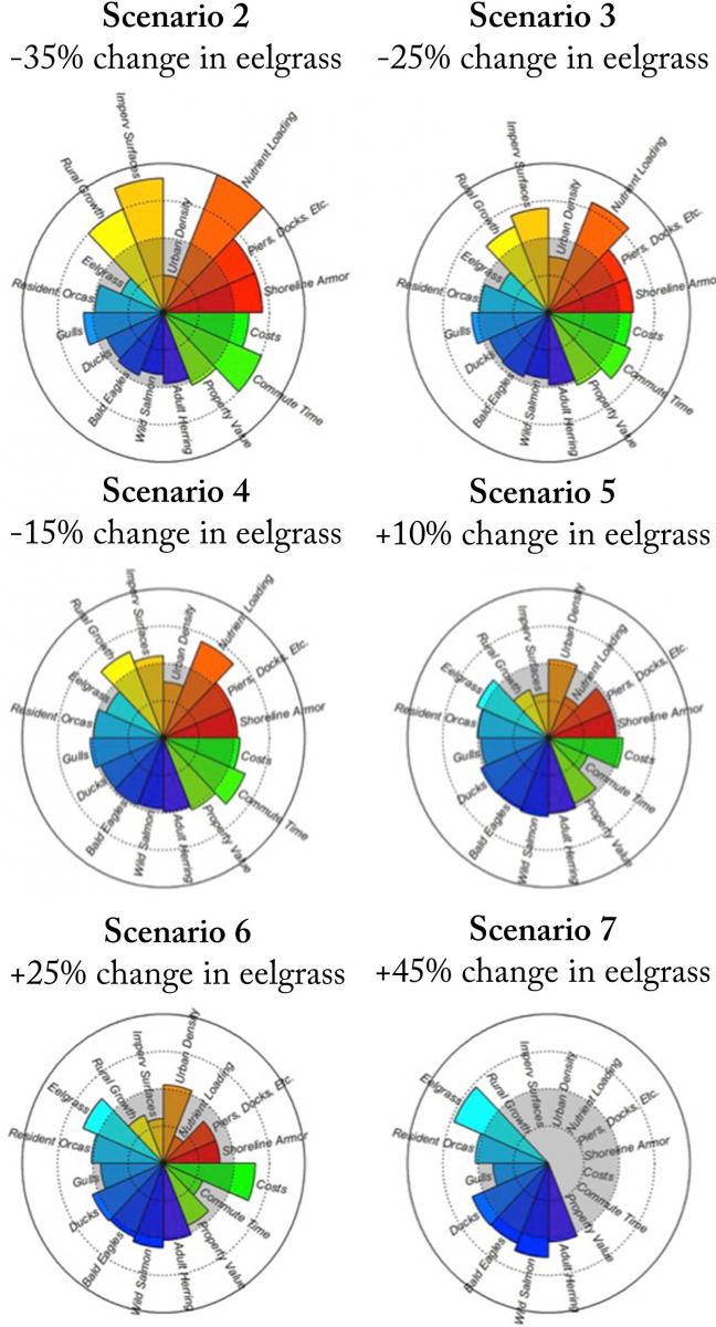
Figure 20, adapted from Levin et al. 2015 with permission. Below is an example of radar plots which were used by Levin and co-authors to show relative trade-offs among 16 different attributes for 6 scenarios related to changes in eelgrass habitat, land use, and shoreline development. Values are plotted relative to the status quo (scenario 1), which is depicted as the gray circle in each plot. Biological ecosystem components are shown in blue; costs are in green; yellow, orange, and red depict anthropogenic pressures and some geographic attributes of the region.
Seagrass loss in Florida
Florida Bay is home to vast stretches of productive seagrass beds that serve as nursery grounds for juvenile fishes and food and habitat for many other marine species. In the 1980s, changes in upstream land uses critically lowered the amount of fresh water supplied to the bay (Rudnick et al. 2005). Less fresh water led to increased concentrations of salt and decreased circulation, agricultural discharges resulted in higher nutrient inputs, and the lack of storms and declines in sea turtle and other wildlife populations may have altered ecosystem dynamics. The interaction of these factors led to a mass die-off of seagrass, affecting 30% of the entire seagrass community, lowering oxygen in the water, and resulting in a non-linear shift between clear water and turbid water in some areas of the Bay. In response, managers at the South Florida Water Management District (SFWMD) launched the first restoration and monitoring efforts in 1992. However, competing scientific hypotheses for the mechanisms of seagrass die-off made it challenging to identify the key drivers and mitigate ecosystem change (Gunderson 2001). After years of experimenting with various potential drivers, the SFWMD created the Minimum Flows and Levels program to maintain freshwater delivery and restore the seagrass ecosystems of the bay. They set a minimum threshold of freshwater input of 105,000 acre-feet of water over a 365-day period, based on the relationship between these drivers, water clarity and seagrass die-offs. For Florida Bay, an exceedance of minimum flow is deemed to occur when the average salinity over 30 or more consecutive days exceeds 30 parts per thousand at the Taylor River salinity monitoring station. If this minimum threshold of freshwater input is breached, upstream municipal and agricultural water uses are prohibited until water delivery is restored.These minimum flow levels are subject to review and revision, allowing for adaptive management of the system as managers monitor seagrass recovery (Madden et al. 2009). As a result of the program, seagrass was restored and has been maintained in Florida Bay over the past decade. However, recent spikes in temperature are putting pressure on the system, indicating the need to revisit the key drivers in the face of a changing climate (see figure below for more details).
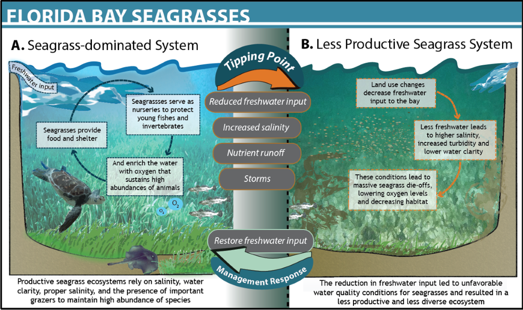
Figure 21, Credit: Ocean Tipping Points Project. Design by: Jacklyn Mandoske.
Oyster die-offs in Pacific Northwest
In the Pacific Northwest oyster farmers began seeing massive die-offs of up to 80% of their oyster larvae, or “seed” beginning in 2005 (Grossman 2011). Recognizing the threat of acidification to the regional economy, local culture, and coastal environment, commercial oyster fisheries began investing in research to better understand the underlying cause of the massive die-offs of oyster larvae. Researchers identified ocean acidification as the major cause of the massive mortality events between 2005 and 2009 (Barton et al. 2012). Following this finding, the federal government further invested $500,000 in monitoring equipment for coastal seawater in order to acquire real-time data on ocean conditions (NOAA 2011). This reaThis real-time monitoring allowed oyster growers to identify when coastal seawater aragonite saturation state (a key parameter of seawater carbonate chemistry) exceeds a critical threshold value of ~1, at which larval growth and shell development are compromised (Waldbusser et al. 2015). Initial solutions have relied on managing around the problem, such as limiting seawater intake to times when conditions are acceptable to young oysters or buffering incoming seawater by adding basic chemicals, such as sodium carbonate (baking soda) (Dewey 2013). However, in the face of global climate change, these solutions are only temporary. Some companies have chosen instead to relocate hatchery operations to more tropical locations less vulnerable to ocean acidification. The collaboration between oyster fishermen and scientists in the Pacific Northwest has resulted in many growers recovering nearly 77% of their losses (see figure below for more details).
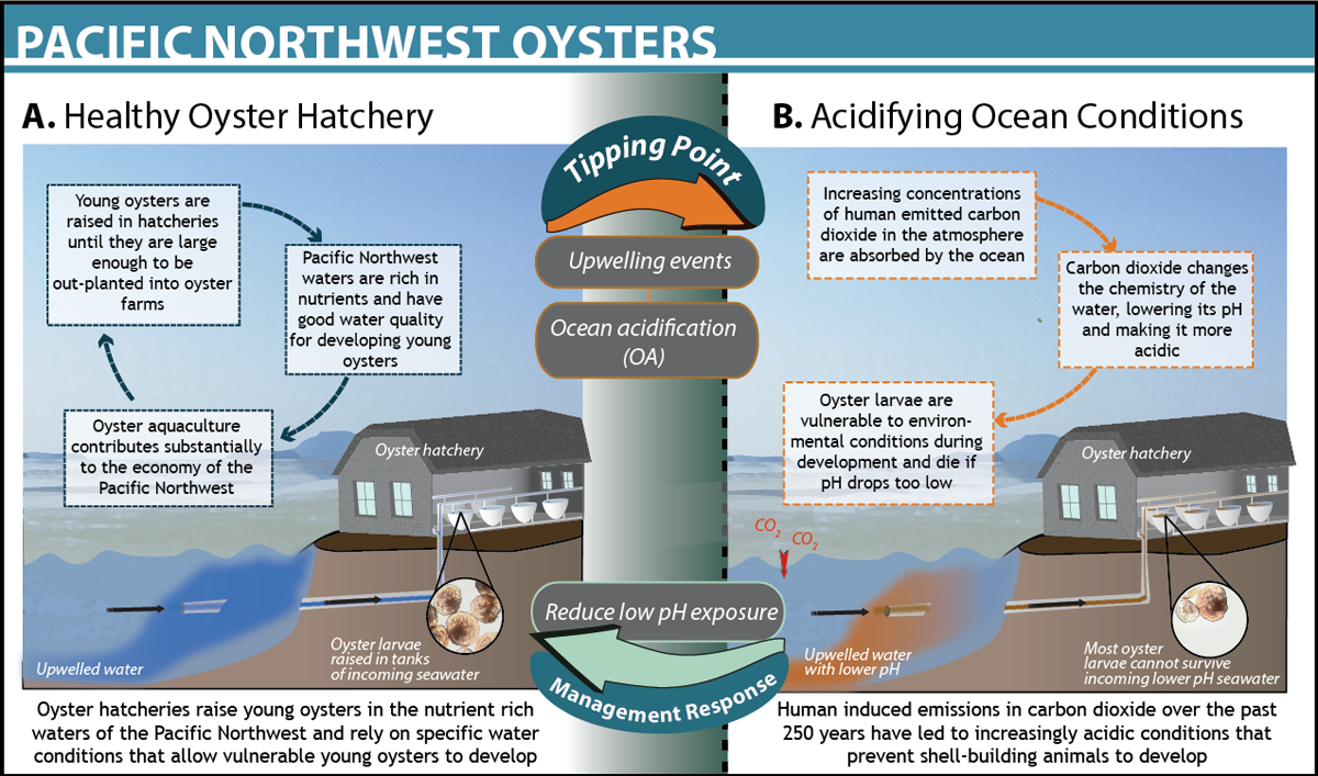
Figure 22, Credit: Ocean Tipping Points Project. Design by: Jacklyn Mandoske.