
Strategy 1. Characterize tipping points in your system

"Identifying how and at what level activities and actions lead to ecosystem tipping points is highly relevant to choosing effective management targets and limits" - Selkoe et al. 2015
Strategy 1a. Define tipping points of concern
What does this mean?
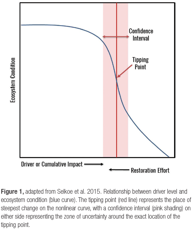
A tipping point is a point of rapid change from one set of conditions to another. In an ecosystem, a tipping point occurs when a small change in environmental or human pressures leads to a large change in components of a social-ecological system and the benefits they provide to people. When crossing these tipping points profoundly affects the entire ecosystem, we refer to them as regime shifts.

Tipping points occur in a wide variety of marine and coastal ecosystem types across the globe, as shown in the figure below. These ecosystem shifts can have large impacts on the social and economic systems that rely upon them.
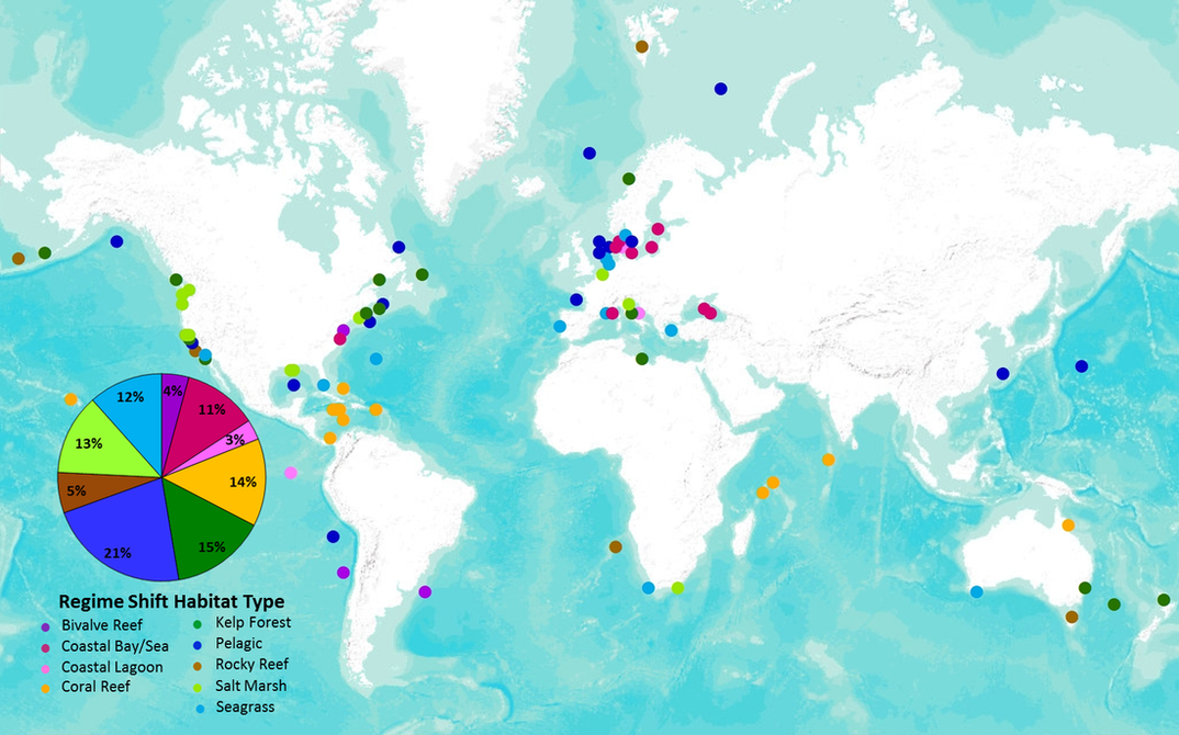
Figure 2, adapted from Kappel et al. in prep. Map of known marine and coastal ecosystem shifts around the world. Note that the higher frequency of regime shifts in temperate waters is probably a reflection of sampling effort as these areas have historically been better studied.
 Social-ecological transitions may be difficult to reverse. When mounting stress disrupts the feedbacks that usually maintain a system in a given state, the system can cross a tipping point and rapidly reorganize into a new state with new feedback mechanisms that reinforce it. This can make it harder, or even impossible to return to the previous state. For example, beginning in the late 1980s, fishermen in Maine took advantage of the boom in sea urchin populations that occurred with the collapse of cod. The aggressive overharvesting of green sea urchins from Maine’s kelp forests resulted in massive declines of urchins along the coast. This overharvesting of sea urchins resulted in another tipping point for the system, shifting from an urchin-dominated patchy kelp forest, to one devoid of sea urchins and teeming with crabs and lobsters that now thrive in the newly established, dense kelp forests. Despite a variety of regulations, managers have not successfully halted or reversed the decline of green urchins. Although monitoring indicated sufficient settlement of sea urchin larvae, experiments have found that crabs have become the new apex predator, consuming sea urchins and their larvae before they can re-establish.
But not all tipping points are negative. In some cases, a tipping point may lead to rapid and dramatic improvements in ecosystem conditions, something that can be critical to understand when planning restoration activities.
Why is it important?
 Scientists, managers, stakeholders, and policy-makers can benefit from considering possible tipping points, whether the context is restoration, fisheries, water quality, or ecosystem-based management.
Our recent review of 51 case studies with ecosystems prone to tipping points showed that, in a variety of settings, management strategies that include monitoring ecosystem state and identifying measurable tipping points tend to be more effective in achieving management goals than strategies that do not consider potential tipping points (Kelly et al. 2014).
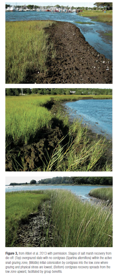
Identifying and characterizing tipping points in your system can help you to avoid crossing unwanted tipping points and enhance your management effectiveness. Understanding tipping points in your management context can also help you recover and restore an ecosystem once a threshold has been crossed. If your system has already crossed a tipping point, getting to a more desirable state will depend upon knowing where the threshold for recovery lies and taking actions that increase your chance of restoring the system. By understanding the feedback mechanisms that maintain the system in the alternate state, managers can prioritize those actions: if you know which mechanisms are maintaining the system in a desirable state, you can take action to protect them; if you know which are keeping the system in an undesirable state, you can take action to disrupt them. For example, in salt marshes of the Eastern United States, cordgrass experienced widespread die-offs due to overfishing of crabs. Snails that would otherwise be kept in check by crabs were released from predation, leading to high grazing pressures on the cordgrass. This caused areas of exposed peat that could not support cordgrass growth. However, cordgrass was able to recover over time. The exposed banks eroded and peat transformed into mud. A new feedback mechanism allowed cordgrass to re-establish: initial colonization by cordgrass ameliorated physical stress, allowing further re-vegetation (Altieri et al. 2013). In this system and others, feedbacks between plants and substrate can play a critical role in rapid, reversible ecosystem shifts.
How do you do it?
Describing ecosystem shifts and characterizing past tipping points can be done both qualitatively and quantitatively. This can be done using data on temporal change (time-series data) or by using spatial data to determine the potential trajectory of systems. Which you use will depend on what data are available and relevant for the system in question. Below we review some of the more widely-used techniques and provide examples for further investigation.
Quantitative Methods:
Advances in statistical techniques and computing power have made it easier than ever to identify nonlinear relationships in data and detect thresholds (see Table in section 1b for review of methods). The first set of methods are univariate correlational analyses, which can be used to fit non-linear relationships between drivers and ecosystem condition to identify how ecosystems change and the potential thresholds of change. Generalized additive models (GAMs) are the most common statistical method used to examine non-linear changes in ecological systems, using effective degrees of freedom, or smoothness of the function, as a measure of the strength of non-linearity. GAMs allow fitting non-linear functions to each predictor, making more accurate predictions for the response variable. The actual threshold or point of inflection can then be identified using second derivatives or change-point analysis (also known as STARS). The latter uses sequential t-tests on the mean or variance to detect significant changes in the slope of the relationship between a driver and an ecosystem response.
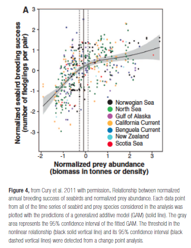 For example, Cury et al. (2011) used GAMs to establish numerical relationships between seabird breeding success and prey abundance and then applied change-point analysis to find the most likely point at which the slope of the relationship changed, i.e., the threshold level of prey abundance that resulted in a rapid change in breeding success (see Figure 2A in Cury et al., 2011 for example of GAM and change-point analysis results). Their analysis resulted in a rule of thumb they called “one-third for the birds,” which provides a simple and quantitative target for managers to consider when evaluating forage fish abundance and determining allowable catch.
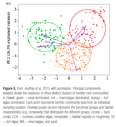 Multivariate methods such as cluster analysis, non-metric multidimensional scaling (nMDS), principal components analysis (PCA), and redundancy analysis (RDA) can also be used to identify ecological communities or regimes that are significantly different from one another. For example, in the Hawaiian archipelago, Jouffray and coauthors (2015) identified coral reef regimes using cluster analysis applied to spatial data on benthic communities (Figure 5 reprinted from Jouffray et al. 2015).
The quantitiative approaches described above and links to examples, publications, code and resources are given at the end of Strategy 1b.
Qualitative Methods:
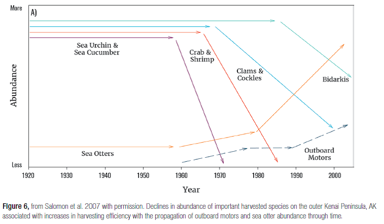
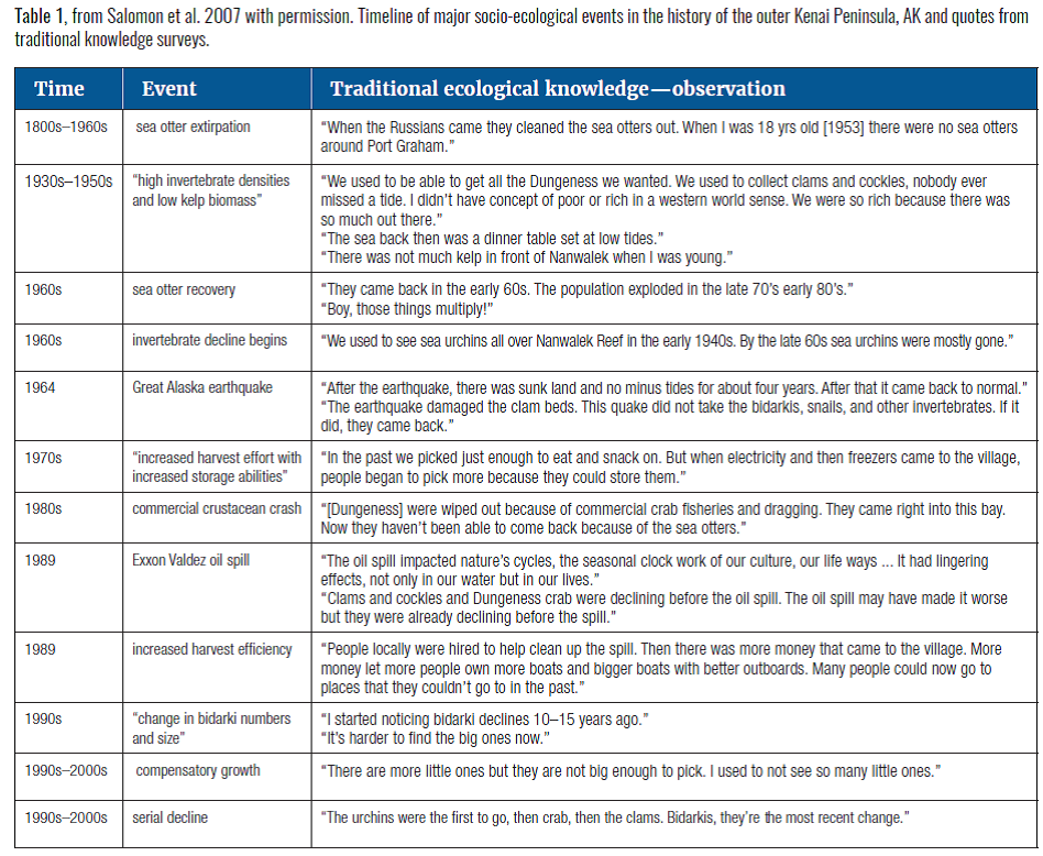
In many systems, quantitative time series are not available to help identify key drivers and describing tipping points. However, traditional and local knowledge can provide a historical perspective to help reconstruct ecosystem changes. For example, Salomon and coauthors (2007) examined the decline of a nearshore benthic invertebrate, the black leather chiton (Katharina tunicata, known locally as Bidarkis), on the rocky shores of the outer Kenai Peninsula, Alaska, USA. This grazing intertidal mollusk has strong top-down effects on seaweeds in the rocky intertidal, and is the basis for a culturally important subsistence fishery for Sugpiaq natives. Using multiple approaches, the authors describe the decline of Katharina and determine the causes. First, they used field surveys to examine the significant predictors of Katharina biomass across 11 sites varying in harvest pressure.
In addition, they analyzed archaeological faunal remains, historical records, traditional ecological knowledge, and contemporary subsistence landings to examine changes in harvest and Katharina biomass over time. Traditional knowledge surveys with Sugpiaq elders and village residents highlighted temporal changes in the relative abundance of invertebrate resources, changes in subsistence use, and sea otter presence from the 1920s to 2003. These data revealed that several benthic marine invertebrates (sea urchin, crab, clams, and cockles) declined serially beginning in the 1960s, co-occurring with recovery of the local sea otter population and increased shoreline harvest efficiency (Figure and Table below from Salomon et al 2007). This work demonstrates the strength of integrating Traditional Ecological Knowledge to reconstruct ecological history and document ecosystem shifts.
Don’t Have Any Data?
If no time-series data are available for the ecosystem in question, or if the historical perspective does not reveal any prior tipping points, it may be useful to look at similar systems in other regions of the world and ask whether tipping points have occurred there and why. The past is not always the best guide to the future in a changing world. Maybe no record of regime shift exists because the drivers of change have been less intense in this region than others. Or perhaps the last big regime shift occurred before living memory. Drawing lessons by analogy to other regions may help you assess the potential risks in the face of data gaps and an uncertain future environment.
For example, while many Pacific reefs are still covered in lush corals and coralline algae, some Pacific reefs and the majority of reefs in the Caribbean have experienced dramatic declines in corals and a phase shift to seaweeds and sponges, driven by a combination of overfishing, land-based runoff, and disease. Managers in other parts of the world are increasingly concerned that amplifying stresses on reefs will lead to similar ecosystem shifts, a pattern that is already starting to emerge.
The Ocean Tipping Points team has assembled a database of tipping points in coastal and marine systems from around the world. By investigating this database along with other literature from similar systems you may gain insights into tipping points that could be crossed in your own system and ways scientists and managers have worked to avoid or recover from them (Kappel et al in prep).
Strategy 1b. Link ecosystem change to key drivers
What does this mean?
Once you have identified the possible tipping points in your system, you will want to determine what factors move the system toward a tipping point. We refer to both the environmental conditions and human activities that can change an ecosystem state as drivers. Effectively managing around these tipping points requires an understanding of the factors driving these changes.
Note: Some texts use terms such as “stressor” or “pressure” in place of “driver,” but this Guide uses “driver,” as this term most broadly captures both natural and anthropogenic factors.
Most studies of the relationships between drivers and ecosystem status focus on individual drivers, and perhaps as a result, many policies and regulations also focus on the management of single drivers (e.g., fishing, pollution, etc.). However, individual drivers may interact to yield surprising results, and it is often the interaction among two or more drivers that leads to a dramatic ecosystem level shift. While scientists are far from being able to predict the outcome of all possible combinations of environmental drivers on marine ecosystems, we do know that the more different drivers are combined, the more likely it is that their combined effect is more than the sum of their individual effects (Crain et al. 2008). And most areas of the ocean are subject to multiple drivers (Halpern et al 2008). For these reasons, it’s important to be alert to cumulative impacts and to test for the effects of multiple drivers simultaneously whenever possible.
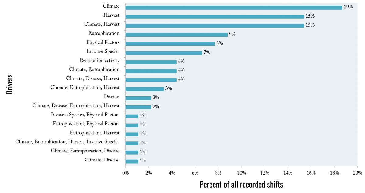
Figure 7, Major pressures and combinations of pressures reported to contribute to observed marine regime shifts around the world based on Kappel et al’s review. Note that these results may be biased toward attributing regime shifts to a single driver, as studies of multiple drivers are limited.
Why is it important?
Identifying the key drivers that can lead (or have led) to a tipping point in your ecosystem is essential to planning a management response. By defining and prioritizing the key drivers acting on the system that are within your management control, you can more clearly define your management objectives and narrow your options for management response.
 Quantifying relationships between drivers and ecosystem responses can help you identify where potential thresholds or tipping points may occur and refine your monitoring plans and targets. In some cases, this may reduce costs and effort; for example, if the relationship between drivers and a tipping point is known, monitoring should be intensified when the system appears close to a tipping point, but could be reduced when far from the tipping point (Stier et al. in prep). Thresholds can inform target setting for management by providing concrete information about system limits, helping to simplify debate about how much human activity is acceptable (Samhouri et al, 2012) and move such debates toward a more objective basis. For example, in the Caribbean, Ocean Tipping Points colleagues (Karr et al. 2015) have shown that a suite of coral reef ecosystem changes is associated with fish densities below 30% of unfished levels: the ratio of macroalgae to coral is higher, the proportion of herbivorous fish in the fish community is lower, and coral cover is much lower suggesting that a tipping point has been crossed. Similar results were obtained in a study of Indian Ocean coral reefs (McClanahan et al 2011). Knowing the driver levels at which such dramatic changes are likely to occur can inform management target setting. Management targets should be informed by these thresholds, as well as influenced by people’s social preferences and how much risk a society is willing to take in their management decision-making. These are discussed in more detail later in this Guide, see strategy 3b, “Use social preferences, risk tolerance and social and ecological thresholds to inform target-setting” for more information.
How do you do it?
As with identifying whether there is a tipping point of concern in your system (Strategy 1a), both qualitative and quantitative methods can be applied to identify potential drivers of change.
Quantitative Methods:
Many of the same statistical techniques that can help you identify tipping points in your system can also be employed to further help you identify the major drivers of these ecosystem changes. Generalized additive models (GAMs) can be used to fit non-linear relationships between drivers and ecosystem condition to identify key drivers of change and potential management levers.
Multivariate statistical tests such as principal components analysis (PCA) and redundancy analysis (RDA) also can be used to examine relationships between drivers and ecological responses. As described in section 1a, these techniques are also useful for identifying regime shifts, and, in combination with change point approaches, determining thresholds in multivariate datasets.
For example, scientists have identified regime shifts in the Central Baltic by applying PCA to environmental time-series data to determine key periods of ecosystem change, followed by STARS to identify the threshold (Möllmann et al. 2009; Tomczak et al. 2013). The analysis identified key drivers of change in the food web, which included a shift in the North Atlantic Oscillation (NAO) that altered thermal, salinity, and nutrient regimes, along with overfishing. The combination of climate- and human-induced drivers on the Baltic Sea ecosystem resulted in new species interactions that led to feedbacks that prevented the recovery of cod, even after hydrological conditions were favorable for cod larvae.
Other multivariate methods like boosted regression trees are also being used to identify direct and indirect effects of drivers on ecosystem components (Elith et al. 2008; Jouffray et al. 2015). While these approaches can be used to identify drivers and quantify thresholds, one disadvantage is that they are correlative and so they are not able to tell you about directionality (e.g., fishing effort could both influence and be influenced by ecosystem condition).
Redundancy analysis is another multivariate approach that can examine non-linear relationships between drivers and ecological responses (Makarenkov and Legendre, 2002; Borcard et al. 2011). Perry and Masson (2013) used RDA to analyze regime shifts in the Salish Sea. They identified a set of six explanatory variables (Chinook salmon hatchery releases, recreational fishing effort, human population size, sea surface temperature, wind, and the North Pacific Gyre Oscillation index) as good predictors of regime shifts. One limitation, however, is that RDA cannot address temporal correlation in datasets.
There are additional multivariate approaches that are better suited to detect patterns in time-series data. For example, dynamic factor analysis (DFA) is a dimension-reduction technique that can be used to examine relationships between response and explanatory variables (Zuur et al. 2003). Scientists have applied DFA to compare trends across ecosystems (Link et al., 2009) and to identify the major drivers of ecosystem changes, such as relationships between warmer sea surface temperatures and higher salmon abundance in the Gulf of Alaska and eastern Bering Sea (Stachura et al. 2013).
Multivariate autoregressive state-space models (MARSS) can be used to examine how non-linear responses in ecosystems are related to biotic processes and changes in external drivers across space and time (Hampton and Schindler, 2006). The strength of MARSS models is that they can focus attention on key drivers of community change and quantify interaction strengths among drivers.
Choosing among these models will depend on the question of interest, the data type, and model assumptions.. We describe the strengths, weaknesses, and additional examples of application in the table below. These methods are explored in more detail in Foley et al (2015).
Summary of quantitative analyses for identifying tipping points of concern and the drivers of change
Generalized additive model (GAM) |
|
| Output | Identifies shape and strength of non-linear relationships between ecological condition and ecosystem driver(s) |
| Strengths | Identifies key drivers |
| Flexible in its ability to fit any shape relationship | |
| Weaknesses | Correlative |
| No directionality of relationships | |
| Computationally complex | |
| May overestimate degree of nonlinearity if overfitting is not controlled | |
| More information & examples | Hastie and Tibshirani (1990), Guisan et al. (2002) |
| Software & code examples | gam package for R |
Change point analysis (e.g., Sequential t-test on the mean, STARS) |
|
| Output | Identifies point of inflection in relationship between ecological condition and ecosystem driver(s), i.e. the threshold |
| Strengths | Identifies location of the threshold or regime shift and corresponding driver/pressure level |
| Identifies leading and lagging indicators | |
| Weaknesses | Correlative |
| No directionality of relationships | |
| Does not explicitly take autocorrelation into account | |
| More information & examples | Rodionov (2006), Cury et al. (2011), Matteson and James (2014), Karr et al. (2015) |
| Software & code examples | VBA for Excel at www.BeringClimate.noaa.gov and strucchange, changepoint, cpm, bcp packages for R |
Redundancy analysis (RDA) |
|
| Output | Identifies non-linear relationships between ecological condition and ecosystem driver(s) |
| Determines likelihood of regime shift | |
| Strengths | Accommodates multivariate datasets |
| Identifies regime shifts | |
| Weaknesses | Correlative |
| No directionality of relationships | |
| More information & examples | Makarenkov and Legendre (2002), Borcard et al. (2011) |
| Software & code examples | rda function in vegan: community ecology R package |
Principal components analysis (PCA) |
|
| Output | Identifies key periods of ecosystem change and associated driver(s) |
| Strengths | Accommodates multivariate datasets |
| Facilitates linking time of ecosystem change to driver number and level | |
| Does not require a priori hypothesis of regime shift year(s) | |
| Weaknesses | Correlative |
| No directionality of relationships | |
| No statistical significance of relationships | |
| More information & examples | Hare and Mantua (2000), Möllmann et al. (2009), Tomczak et al. (2013) |
| Software & code examples | princomp and prcomp in the R Stats package |
Boosted regression trees |
|
| Output | Identifies potentially significant direct and indirect effects of drivers on ecosystem components |
| Strengths | Identifies indirect effects |
| Facilitates experimental and observational studies of ecosystem effects | |
| Weaknesses | Correlative |
| No directionality of relationships | |
| More information & examples | De’Ath (2007), Elith et al. (2008) |
| Software & code examples |
gbm R package |
Qualitative Methods:
Literature Review:
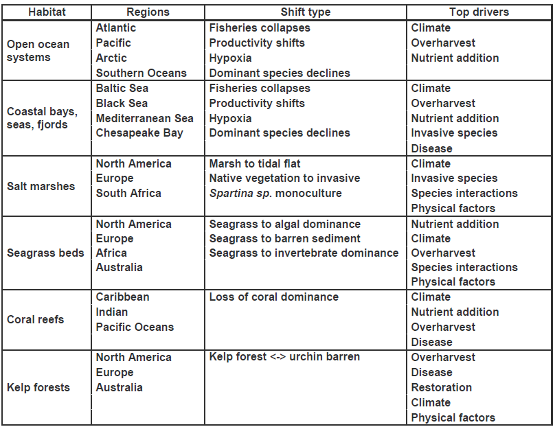
Building off of other available work can also be a good place to start identifying potential drivers when long-term or spatially robust data are unavailable. The Ocean Tipping Points project’s ecosystem shifts database documented 91 regime shifts across all major ocean basins, and nine different marine ecosystem types from the coastal zone to the open ocean (Figure 8, Kappel et al in prep). We also identified the major drivers of these shifts. The most commonly cited drivers include climate change, eutrophication, and changes in harvest rates. By looking at similar ecosystems you may be able to draw preliminary conclusions about potential drivers of concern for your own system.
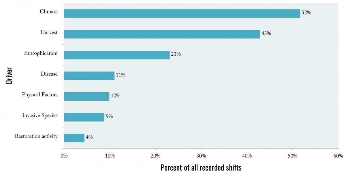
Figure 8, adapted from Kappel et al. unpublished data. Top drivers of 91 marine ecosystem regime shifts from around the world
Expert Knowledge:
Conceptual models provide a framework for understanding ecosystems holistically. Conceptual models represent ecological and/or social components and how they link to one-another, often with a focus on food web relationships. These models may also depict biophysical conditions and potential external drivers (e.g., nutrient input or shifting ocean temperatures) that are most likely to influence or alter those relationships. The information used to build conceptual models can be gathered via literature review and/or through local and expert knowledge.
For example, in Haida Gwaii, British Columbia, Stier and coauthors (2016) elicited experts’ conceptual models of the herring-centric food web from a set of experts (Figure 9, adapted from Siter et al. 2016). These models were then used in network analysis to explore potential implications of various environmental drivers and management decisions.
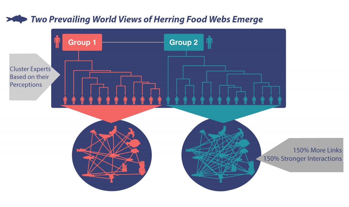
Figure 9, adapted from Stier et al. 2016 with permission. Experts clustered into two groups based on their view of the Haida Gwaii foodweb with herring at its center. Group 1 saw the food web as simpler, with fewer, less strong connections. Group 2 viewed the food web as more complex, with more and stronger linkages among species. Neither demographics, professional affiliation, nor years of experience explained these differences.
Similar to conceptual models, many management agencies are using influence diagrams such as Pathways of Effects approaches to identify potential drivers or combinations of drivers that might influence the system of interest. These influence diagrams are conceptual tools that illustrate the potential cause-and-effect relationships among socio-economic, cultural, and ecological dimensions of a system or problem. Such influence diagrams can be constructed with stakeholder input. This is an important step for characterizing what matters to different groups and how such things might be affected directly or indirectly by management decisions (Chan et al. 2012). Constructing these diagrams with local knowledge holders can help identify differences in perception within the community that can be further explored or addressed. For example, if the differences in perception are based on a lack of awareness of scientific information, improved education and outreach can foster shared understanding. Alternatively, such differences can point to areas of critical scientific uncertainty for further research. In addition, divergent stakeholder views or risk tolerances can be included explicitly in decisionmaking processes (e.g., by illustrating tradeoffs in what different people care most about). Working with stakeholders to construct an influence diagram or system map can be an effective way to draw on local knowledge, empower participants, and generate common understandings of the system so as to reduce conflict and enhance communication.
Quantitative, semi-quantitative and qualitative methods can then be applied to these linkage diagrams to further explore consequences of decisions. Examples include structural equation modeling (SEM), Bayesian belief network analysis, loop analysis, and fuzzy cognitive models. For example, Martone and colleagues (2017) developed a simplified diagram of the social-ecological connections in small-scale fisheries of Baja California, Mexico. Using qualitative loop analysis, the authors identified potential social and ecological consequences of natural perturbations and management decisions on a coastal fishery, and identified which drivers and pathways may have greater influence on the outcomes, highlighting potentially important relationships to examine in future research and analysis.
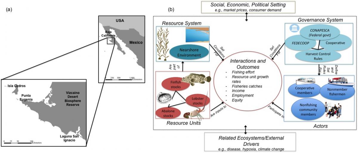
Figure 10, from Martone et al. 2017 with permission. The fishing cooperatives of the Vizcaino region in Baja California Sur, Mexico: (a) map of the study area showing location along the coastline from Punta Eugenia to Laguna San Ignacio; (b) conceptual representation of the social-ecological system (SES) based on the updated SES framework presented in McGinnis and Ostrom (2014).